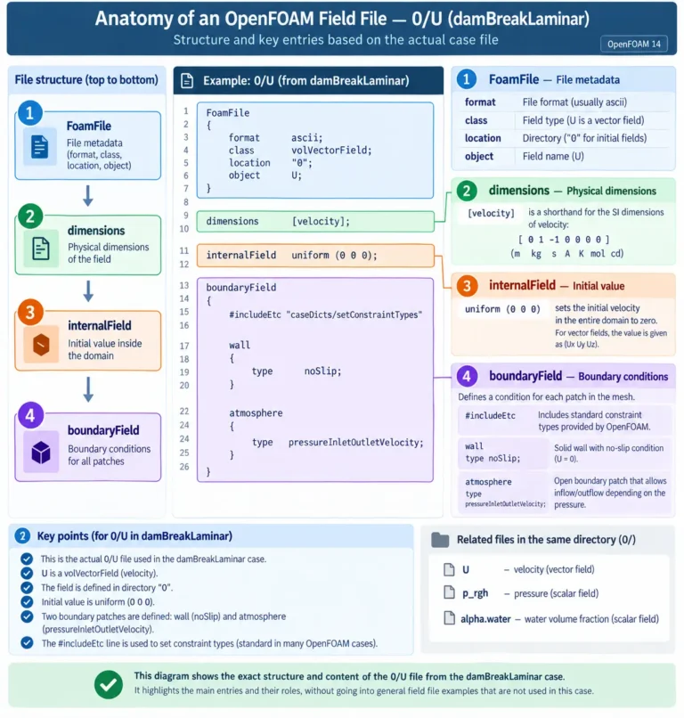

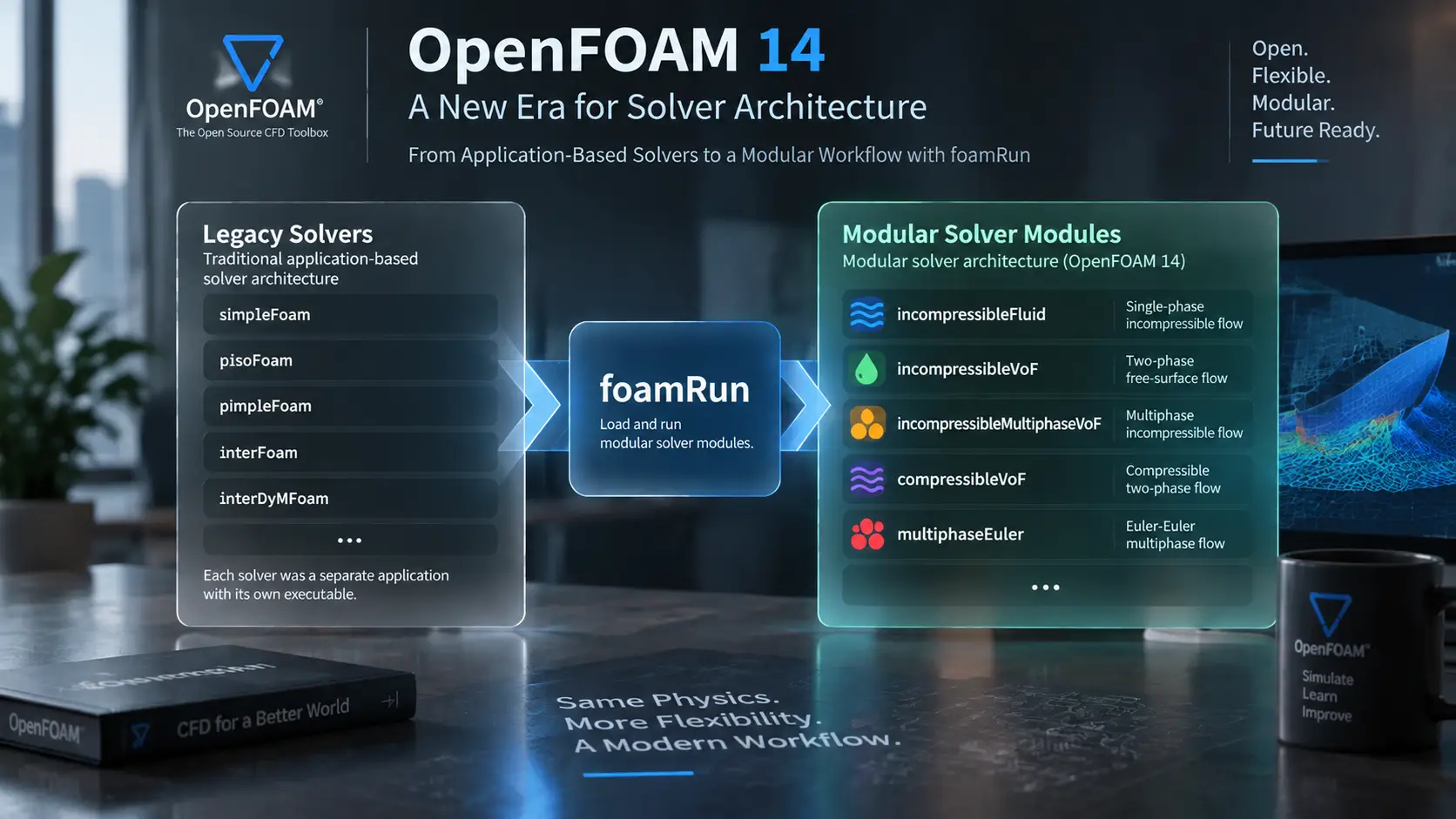
OpenFOAM 14 Solver Architecture: Transitioning from Application-Based to Modular CFD Workflows
This article examines the transition from traditional OpenFOAM solver applications toward modular CFD workflows, explains the role of foamRun and solver modules, and demonstrates the architecture using the DTC HullWave marine CFD case as an engineering example.
1. Introduction: Why Solver Architecture Matters in OpenFOAM
OpenFOAM is a CFD framework built around flexibility, transparency, and direct user control over the simulation workflow. Unlike many commercial CFD platforms where the numerical process is managed through predefined interfaces, OpenFOAM exposes the major components involved in a CFD calculation. Users define the computational domain, physical models, numerical schemes, boundary conditions, and solution controls through case configuration files.
For this reason, understanding OpenFOAM requires more than knowing how to execute a simulation. A reliable CFD workflow depends on understanding how different parts of the software architecture interact and how the selected computational framework transforms a mathematical model into a numerical solution.
A typical OpenFOAM case is organized around three main directories:
case/
0/constant/system/The 0 directory contains initial fields and boundary conditions.
The constant directory defines mesh information, physical properties, and modelling parameters.
The system directory controls runtime settings, numerical schemes, and solution procedures.
For a detailed explanation of OpenFOAM case organization and directory structure, see our OpenFOAM 14 Case Structure Guide.
However, the case structure alone does not explain how OpenFOAM determines the computational framework responsible for solving the governing equations. This requires understanding another important layer of the workflow: solver architecture.
Solver architecture defines how OpenFOAM connects the mathematical formulation of a CFD problem with the numerical procedures required to obtain a solution. It determines the relationship between:
- governing equations,
- pressure-velocity coupling,
- physical models,
- numerical algorithms,
- time advancement procedures.
Historically, OpenFOAM users interacted with this architecture through dedicated solver applications. The selected executable represented a complete computational workflow designed for a specific category of CFD problem.
Common examples include:
simpleFoamfor steady incompressible turbulent flows,pimpleFoamfor transient incompressible simulations,interFoamfor incompressible two-phase Volume of Fluid (VOF) simulations,interDyMFoamfor multiphase simulations involving dynamic mesh motion.
Users beginning with OpenFOAM workflows can also explore our practical OpenFOAM 14 PitzDaily Steady Tutorial.
In this traditional approach, the solver application was closely associated with the physical problem being simulated.
For example:
interFoamThis application-based workflow became a fundamental part of OpenFOAM usage because it provided a clear relationship between a physical problem and the computational tool required to solve it.
However, modern engineering simulations increasingly involve combinations of multiple physical and numerical requirements. Problems are no longer always represented by a single isolated phenomenon.
A realistic CFD application may involve:
- multiphase interaction,
- turbulence modelling,
- transient behaviour,
- interface tracking,
- moving boundaries,
- complex numerical procedures.
Marine hydrodynamics provides a clear example of this increasing complexity. A ship-wave interaction simulation requires the interaction of several capabilities, including free-surface modelling, turbulence treatment, transient solution methods, and appropriate numerical configuration.
In an application-based architecture, supporting every possible combination of these requirements can lead to an increasing number of specialized solver applications. As the complexity of engineering simulations grows, the relationship between a physical problem and a single predefined solver becomes more difficult to maintain.
OpenFOAM 14 represents an evolution toward a more modular organization of solver functionality. Instead of considering the solver only as a single executable application, the workflow separates different computational responsibilities.
The general concept can be represented as:
The purpose of this evolution is not to change the fundamental principles of CFD. Governing equations, numerical accuracy, physical modelling, and validation remain the foundation of every simulation. The main change is how different computational responsibilities are organized within the software framework.
For existing OpenFOAM users, this introduces a different way of thinking about solver selection.
The traditional question:
Which solver application should I run?
becomes a broader question:
Which computational capabilities does my physical problem require?
This article examines the transition from traditional OpenFOAM solver applications toward modular CFD workflows, explains the role of foamRun and solver modules, and demonstrates the architecture using the DTC HullWave marine CFD case as an engineering example.
2. Traditional OpenFOAM Solver Architecture
Before examining the modular solver workflow, it is important to understand the traditional solver architecture that shaped OpenFOAM usage for many years.
In the application-based approach, the solver application acted as the main computational entry point of a simulation. Users selected an executable that already represented a specific category of CFD problem and contained the required solution framework.
The traditional workflow was:
The traditional OpenFOAM architecture was built around dedicated solver applications, where each executable represented a complete numerical workflow for a specific class of CFD problems.
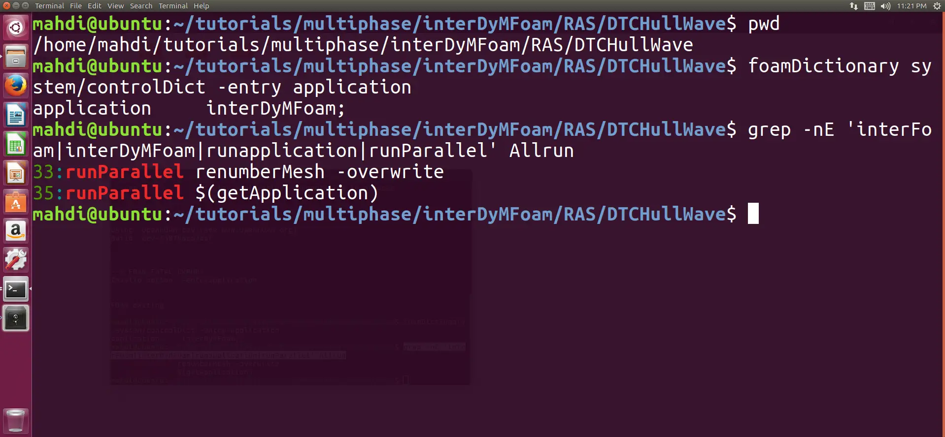
The selected solver application connected several computational components, including:
- governing equations,
- numerical algorithms,
- physical models,
- time advancement procedures,
- solution controls.
Although users configured many aspects of the simulation through OpenFOAM dictionaries, the overall computational structure was determined by the selected solver application.
This approach created a clear relationship between engineering problems and computational tools. Users learned OpenFOAM workflows by associating specific solver applications with specific classes of simulations.
simpleFoam: Steady Incompressible Flow
simpleFoam represents the traditional workflow for steady incompressible turbulent flow simulations.
Typical applications include:
- external aerodynamics,
- internal flow systems,
- industrial ventilation,
- steady engineering calculations.
The solver is based on the SIMPLE algorithm for pressure-velocity coupling.
A simplified representation is:
The application provided the solution framework, while users defined:
- turbulence models,
- fluid properties,
- boundary conditions,
- numerical schemes.
pimpleFoam: Transient Incompressible Flow
For transient incompressible simulations, users commonly selected pimpleFoam.
Unlike steady-state calculations, transient CFD requires solving the governing equations repeatedly over a sequence of time steps.
The PIMPLE algorithm combines features of SIMPLE and PISO methods to manage pressure-velocity coupling during transient calculations.
Typical applications include:
- unsteady aerodynamic flows,
- transient industrial systems,
- time-dependent engineering problems.
The solver application managed:
- time advancement,
- pressure correction,
- iterative solution procedures.
interFoam: Free-Surface and Multiphase Flow
interFoam became one of the most recognized OpenFOAM solvers for free-surface simulations.
It is based on the Volume of Fluid (VOF) approach, where the interface between immiscible fluids is represented through a phase fraction field.
Typical applications include:
- water-air free surfaces,
- wave propagation,
- ship hydrodynamics,
- tank sloshing.
A simplified representation is:
The important characteristic of this solver was the integration of several capabilities within one application:
- incompressible flow,
- multiphase modelling,
- interface capturing,
- numerical solution procedures.
interDyMFoam: Multiphase Flow With Dynamic Mesh
Some engineering problems require both multiphase modelling and changing computational geometry.
Examples include:
- ship motion,
- rotating machinery,
- moving boundaries.
interDyMFoam combined VOF-based multiphase capabilities with dynamic mesh functionality.
This example demonstrates a key characteristic of the traditional architecture:
When new combinations of physics appeared, additional solver applications were often required.
This approach was effective when CFD problems could be represented by a limited number of predefined categories. However, as engineering simulations became increasingly complex and multiphysics problems became more common, maintaining a separate application for every possible combination became more difficult.
This limitation motivated the transition toward a more modular solver architecture, discussed in the following section.
3. Why Application-Based Solver Architecture Became Limited
The traditional solver architecture provided OpenFOAM users with a clear and practical workflow. Selecting a solver application usually meant selecting a complete computational framework designed for a specific class of CFD problem.
This approach was effective when engineering simulations could be represented by a limited number of predefined categories. However, as CFD applications became more complex, the relationship between a physical problem and a single solver application became increasingly difficult to maintain.
Modern engineering simulations often require multiple interacting physical capabilities. A single simulation may involve combinations of:
- incompressible flow,
- turbulence modelling,
- multiphase interaction,
- interface tracking,
- moving boundaries,
- transient solution procedures.
A marine hydrodynamics simulation is a representative example. A ship-wave interaction problem may require:
- free-surface modelling,
- VOF interface tracking,
- turbulence modelling,
- wave boundary conditions,
- transient solution methods.
In an application-based architecture, supporting every possible combination of these requirements can lead to an increasing number of specialized solver applications.
3.1 Increasing Number of Specialized Solvers
Each traditional solver application represents a predefined combination of physical and numerical capabilities.
Examples include:
simpleFoaminterFoaminterDyMFoamEach application provides a complete workflow for a specific problem category.
However, as new physical requirements are introduced, the number of possible combinations increases rapidly.
A simulation requiring:
- incompressible flow,
- VOF interface tracking,
- turbulence,
- mesh motion,
- additional physical models,
- may require functionality from several different solver categories.
The challenge is not implementing these individual capabilities. The challenge is maintaining a software structure where increasing combinations remain manageable.
3.2 Code Coupling and Maintenance Challenges
Another limitation of application-based architecture is the strong connection between execution logic, physical modelling, and numerical procedures.
A traditional solver application often combines several responsibilities:
Different solver applications may require similar functionality, including:
- pressure-velocity coupling,
- transport equations,
- turbulence models,
- numerical methods,
- boundary condition handling.
When these components are tightly connected inside separate applications, extending the framework becomes more difficult.
A modification or improvement affecting a common component may require additional consideration across multiple solver implementations.
The challenge is therefore not only code duplication, but also the difficulty of maintaining clear separation between different computational responsibilities.
3.3 Difficulty Supporting Multiphysics Applications
Modern CFD increasingly involves problems where several physical processes interact.
Marine hydrodynamics provides a clear example.
A ship-wave interaction simulation may require:
- free-surface modelling,
- multiphase interface tracking,
- turbulence modelling,
- transient solution procedures,
- moving geometry or mesh motion.
Representing every possible combination of these requirements through separate solver applications becomes increasingly difficult as the number of available physical models grows.
The limitation of the traditional architecture is therefore related to software organization rather than CFD capability.
The governing equations, physical models, and numerical methods remain essential. The challenge is how these components are organized and combined within the solver framework.
These limitations created the need for a more flexible organization of solver functionality, leading toward the modular architecture discussed in the following section.
4. The Transition Toward Modular Solver Architecture
The limitations of application-based solver architecture created the need for a more flexible way of organizing CFD capabilities. As engineering simulations became more complex, connecting an entire physical problem to a single solver executable became increasingly difficult to maintain.
The goal of modular solver architecture is not to replace CFD fundamentals or change the mathematical principles behind numerical simulation. Governing equations, physical modelling, numerical accuracy, and validation remain the foundation of every CFD workflow.
The main change is the organization of computational responsibilities.
In the traditional approach:
The solver application acted as the central component connecting the physical problem with the numerical solution.
In a modular workflow, these responsibilities are separated into different layers:
Each layer has a defined role within the simulation process.
This separation allows OpenFOAM to organize solver functionality in a more flexible way while preserving the fundamental principles of CFD.
4.1 Separation Between Execution and Physics
The most important conceptual change in modular solver architecture is the separation between:
- how a simulation is executed,
- what physical problem is being solved.
In traditional solver applications, these responsibilities were combined.
For example, interFoam represented a complete workflow for incompressible multiphase VOF simulations. The application connected:
- execution procedure,
- numerical solution process,
- multiphase formulation,
- required physical components.
The modular approach separates these responsibilities.
The execution framework provides the mechanism required to run the simulation, while the solver capability defines the computational framework required for a specific class of CFD problems.
Conceptually:
This separation creates clearer boundaries between different parts of the CFD workflow.
4.2 From Solver Applications to Solver Capabilities
One of the main changes introduced by modular architecture is the way solver selection is understood.
In the traditional workflow, users often started with an application name:
interFoamThe solver application represented the complete computational environment.
In the modular workflow, the starting point is the physical requirement:
The focus shifts from remembering executable names toward identifying the capabilities required by the simulation.
This change becomes increasingly important for complex engineering problems where several computational requirements must interact.
The user moves from a solver-centered perspective toward a capability-centered perspective.
4.3 Organizing CFD Functionality Into Separate Layers
A modular architecture separates different aspects of a CFD calculation rather than combining all responsibilities inside a single application.
A complete simulation can be viewed as the interaction of several layers:
Each layer contributes a specific role.
The solver capability defines the computational framework required for the problem class.
Physical models describe the behaviour of the simulated system.
Numerical methods determine how the governing equations are transformed into a computational solution.
This organization improves flexibility because individual components can evolve without requiring every possible combination to become a separate solver application.
4.4 Supporting Complex CFD Workflows
The importance of modular organization becomes clearer as CFD problems involve increasing numbers of interacting requirements.
A simple simulation may involve a limited set of capabilities:
More advanced engineering simulations may require several interacting components:
The challenge is not the ability to solve these individual physical processes.
The challenge is organizing them in a way that allows different capabilities to work together without creating a new solver application for every possible combination.
This is one of the main motivations behind modular solver architecture.
4.5 Relationship Between Case Structure and Modular Architecture
An important aspect of the transition is that modular solver architecture does not replace the traditional OpenFOAM case structure.
The familiar directories remain the foundation of the simulation:
0/
constant/
system/
These files continue to define:
- initial conditions,
- boundary conditions,
- mesh information,
- physical properties,
- numerical settings.
The modular architecture operates above this existing structure.
The relationship can be represented as:
The case defines the engineering problem.
The solver architecture defines how that problem is computationally executed.
4.6 Why This Evolution Matters
The transition toward modular solver architecture represents a change in
software organization rather than a change in CFD methodology.
Users still require knowledge of:
- conservation equations,
- fluid behaviour,
- turbulence modelling,
- multiphase physics,
- numerical stability.
The difference is how these concepts are organized within the computational framework.The traditional workflow encouraged users to think:
The modular workflow encourages a different approach:
This transition provides a more flexible foundation for increasingly complex CFD applications.
The next section examines the execution layer of this architecture and explains the role of foamRun in running solver modules within the modular workflow.
5. What Exactly Is foamRun in OpenFOAM 14?
One of the central concepts in the OpenFOAM 14 modular solver workflow is foamRun. For users familiar with previous OpenFOAM workflows, understanding foamRun requires a change in how solver execution is interpreted.
In the traditional approach, the solver application was the direct entry point of the simulation. Users selected an executable such as:
simpleFoam,pimpleFoam,interFoam.
Each application represented a complete computational workflow containing the required solution structure for a specific class of CFD problem.
The application connected several responsibilities:
- numerical algorithms,
- physical models,
- equation solution procedures,
- time advancement,
- runtime control.
In the modular architecture, these responsibilities are separated.
The workflow becomes:
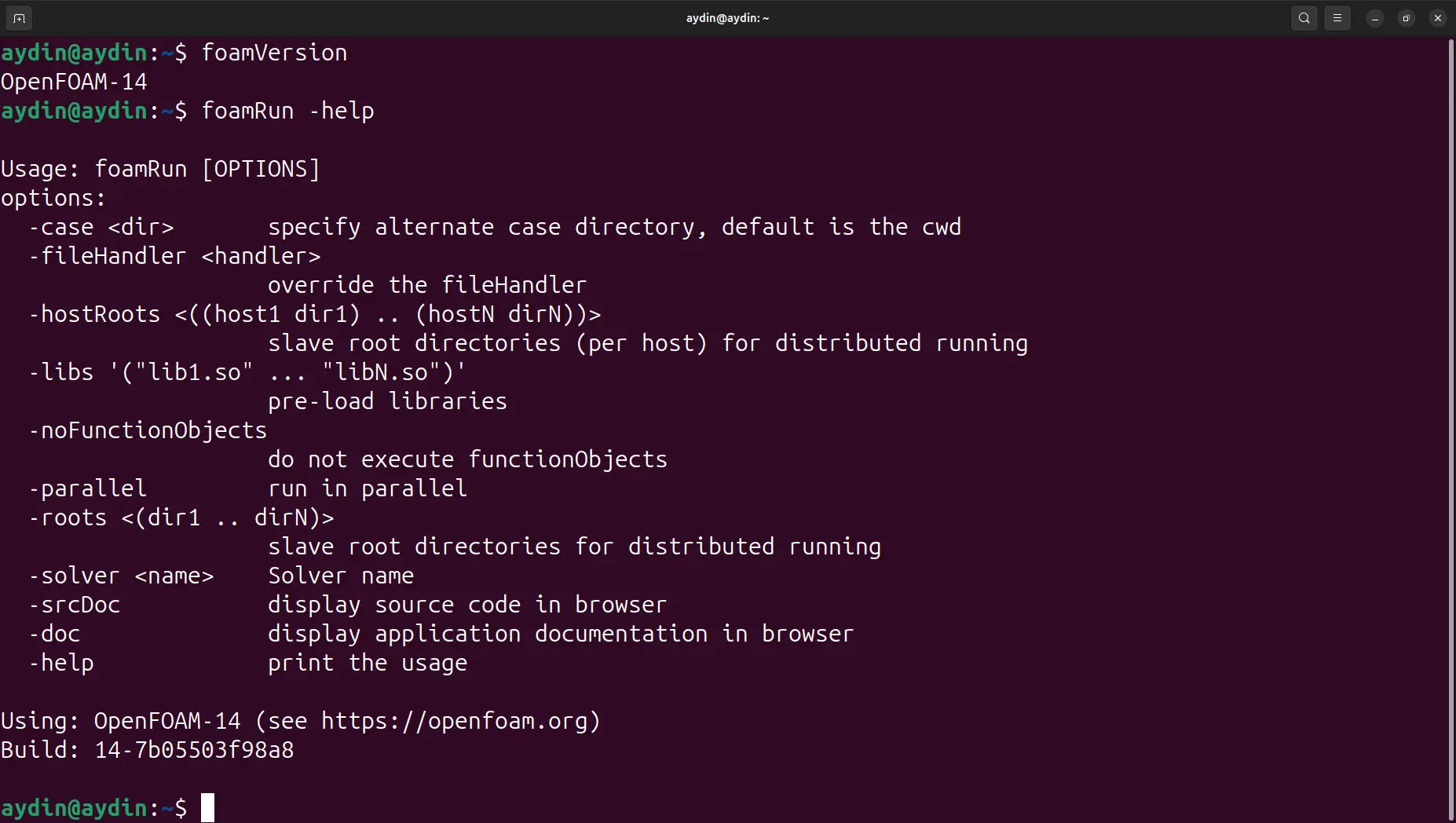
foamRunThe role of foamRun is to provide the execution framework that starts the simulation and connects the OpenFOAM case with the selected solver capability.
5.1 foamRun as the Execution Framework
foamRun should be understood as an execution mechanism rather than a traditional CFD solver.
Its main responsibility is managing the execution process and loading the selected solver module.
It does not define the physical nature of the simulation.
For example, foamRun itself does not determine:
- whether the flow is incompressible,
- whether multiple phases exist,
- whether turbulence modelling is required,
- whether a free surface is present.
These decisions belong to the selected solver capability and associated physical models.
The relationship is:
foamRunTherefore, foamRun represents a change in software organization rather than a new solver category.
5.2 foamRun and the Separation Between Execution and Physics
The main difference between traditional solver applications and the modular workflow is the separation between execution and physics.
In the traditional architecture:
The application combined execution logic with the physical capability required for the problem.
In the modular workflow:
The execution mechanism and the physical definition of the problem are handled by separate components.
This separation allows different capabilities to be organized and extended independently.
OpenFOAM 14 introduces a different execution philosophy where the runtime framework and the numerical capabilities are separated.
5.3 How foamRun Fits Into the OpenFOAM Workflow
foamRun does not replace the OpenFOAM case structure.
The simulation still begins with the case definition:
0/
constant/
system/
These files continue to define:
- initial and boundary conditions,
- mesh information,
- physical properties,
- numerical settings.
The relationship becomes:
foamRun ExecutionThe case describes the engineering problem.
foamRun provides the execution mechanism.
The solver module provides the computational capability required to solve the equations.
5.4 Example: Free-Surface Marine CFD Workflow
Consider a marine CFD simulation involving ship motion and free-surface waves.
The physical requirements may include:
- incompressible water flow,
- air-water interface tracking,
- VOF modelling,
- turbulence treatment,
- transient solution procedures.
The traditional interpretation would focus on selecting a solver application:
interFoamThe modular interpretation focuses on the required computational capability:
foamRunThe focus moves from the name of the executable toward the physical and numerical requirements of the problem.
5.5 Impact on Existing OpenFOAM Users
For experienced OpenFOAM users, the main importance of foamRun is understanding the separation between execution and computational capability. Previously, the solver application represented the complete simulation workflow. Traditional workflow: Solver Application ↓ Complete Workflow ↓ Simulation In the modular workflow: Execution Framework ↓ Solver Capability ↓ Physical Models ↓ Numerical Solution foamRun therefore changes how simulation components are connected rather than changing the underlying CFD principles.
5.6 Summary
foamRun is one of the key components of the OpenFOAM 14 modular solver workflow.
It is not a replacement name for traditional solvers and it is not a universal CFD solver containing all physical models.
Its role is to provide a common execution framework that allows solver modules to be selected and executed independently from the physical capabilities they provide.
Understanding this distinction is essential for understanding how OpenFOAM 14 connects traditional solver concepts with a modular CFD architecture.
6. Solver Modules in OpenFOAM 14
Solver modules are the core building blocks of the modular solver architecture.
In the traditional OpenFOAM workflow, users selected a complete solver application that represented a specific class of CFD problem. In the modular workflow, the focus shifts from selecting an application name toward selecting the computational capability required by the physical problem.
A solver module represents the solution framework required for a particular category of CFD simulations.
It defines the computational structure needed to solve a class of problems, while execution is handled separately through the modular workflow.
The relationship is:
foamRunA solver module should not be considered a direct replacement name for an old solver application.
Instead, it represents a reusable CFD capability that can be combined with other components of the simulation workflow.
6.1 Role of Solver Modules
A CFD simulation consists of multiple interacting layers:
The solver module provides the main computational framework, but it does not completely define the final simulation.
For example, selecting an incompressible flow capability does not automatically determine:
- turbulence model,
- mesh resolution,
- boundary conditions,
- discretization schemes,
- convergence criteria.
These remain part of the case configuration.
Therefore, a solver module should be understood as one layer of the CFD workflow rather than the complete simulation itself.
6.2 incompressibleFluid Solver Module
The incompressibleFluid solver module represents the capability required for incompressible single-phase flow simulations.
Typical applications include:
- internal flow systems,
- external aerodynamic flows,
- industrial flow applications,
- ventilation systems.
The computational framework is based on solving the incompressible flow equations, where pressure and velocity fields are the main solution variables.
A simplified representation is:
The solver module provides the solution framework, while the user defines additional aspects of the simulation, including:
- turbulence modelling,
- transport properties,
- numerical schemes,
- boundary conditions.
6.3 incompressibleVoF Solver Module
The incompressibleVoF solver module represents the capability required for incompressible multiphase simulations using the Volume of Fluid method.
It is particularly important for problems involving a distinct interface between immiscible fluids.
Typical applications include:
- water-air free surfaces,
- ship hydrodynamics,
- wave propagation,
- tank sloshing.
The VOF method represents the interface through a phase fraction field rather than explicitly tracking the interface geometry.
A simplified representation is:
For water-air simulations, the phase fraction field commonly represents the distribution of water inside computational cells.
Conceptually:
alpha.water = 1alpha.water = 0Values between these limits represent cells containing the interface between the two phases.
6.4 Multiphase CFD Capability Selection
Not all multiphase problems require the same modelling approach.
VOF-based methods are typically used when the interface between phases is important.
Examples include:
- free surfaces,
- wave interaction,
- liquid-gas interfaces.
Other problems involve phases distributed throughout the domain.
For these cases, Eulerian multiphase approaches may be more appropriate.
Examples include:
- gas-liquid mixtures,
- dispersed particle flows,
- industrial multiphase processes.
The important point is that solver modules describe the computational capability required by the physical problem.
6.5 Solver Modules as Capability Definitions
The modular architecture changes the way CFD workflows are described.
Traditional thinking:
I need interFoam
Capability-based thinking:
I need:
- incompressible flow
- interface tracking
- VOF multiphase capability
- The focus moves from remembering application names toward understanding the physical requirements of the simulation.
This approach becomes increasingly valuable as engineering problems require combinations of multiple computational capabilities.
6.6 Summary
Solver modules are the main computational components of the OpenFOAM 14 modular workflow.
They define the capability required for different categories of CFD problems while remaining separate from the execution mechanism provided by foamRun.
Examples include:
incompressibleFluidfor incompressible single-phase flow,incompressibleVoFfor VOF-based free-surface simulations,- Eulerian multiphase capabilities for distributed multiphase systems.
The important architectural change is the separation between:
This separation provides a more flexible framework for organizing complex CFD workflows.
7. Mapping Traditional Solvers to Modular Capabilities
The transition from traditional solver applications to modular solver capabilities can create uncertainty for experienced OpenFOAM users.
For many years, users learned OpenFOAM through solver names. Applications such as simpleFoam, pimpleFoam, and interFoam became associated with specific categories of CFD problems.
In the modular workflow, the focus changes from remembering application names to identifying the computational capability required by the physical problem.
This does not mean that traditional solvers lose their importance. They remain useful references because they represent the historical organization of OpenFOAM workflows.
The relationship should be understood as:
This relationship describes functional correspondence, not a direct one-to-one replacement.
7.1 Why Mapping Is Useful
For existing OpenFOAM users, the main challenge is translating previous experience into the modular architecture.
A user familiar with:
interFoam
already understands important concepts such as:
- incompressible multiphase flow,
- VOF interface capturing,
- phase fraction fields,
- free-surface modelling.
The modular workflow does not remove this knowledge.
Instead, it changes how these concepts are organized within the software architecture.
The user moves from:
I know which solver application I need.
toward:
I know which computational capability my simulation requires.
7.2 Traditional Solver to Capability Mapping
The following relationships provide a conceptual connection between traditional solver applications and modular capabilities.
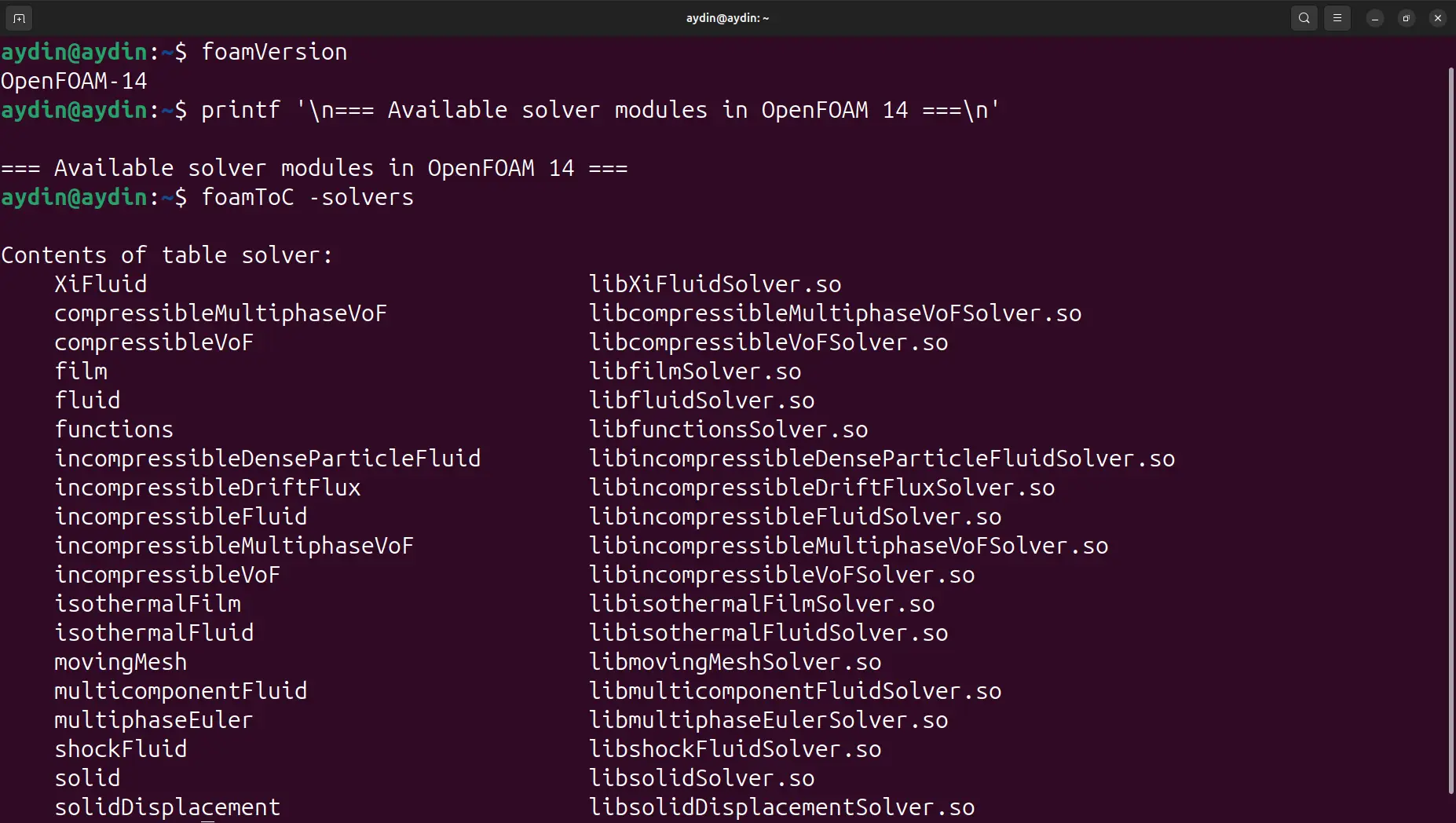
| Traditional Solver | CFD Problem Category | Modular Capability |
|---|---|---|
simpleFoam | Steady incompressible turbulent flow | incompressibleFluid |
pimpleFoam | Transient incompressible flow | incompressibleFluid + transient solution configuration |
interFoam | Incompressible VOF free-surface flow | incompressibleVoF |
multiphaseEulerFoam | Eulerian multiphase flow | multiphaseEuler |
These relationships should be interpreted as capability mapping rather than replacement rules.
7.3 simpleFoam and incompressibleFluid Capability
simpleFoam has traditionally been associated with steady incompressible turbulent flow simulations.
Typical applications include:
- aerodynamic flows,
- internal flow systems,
- industrial fluid applications.
The corresponding modular interpretation is:
incompressibleFluid CapabilityThe important connection is the physical problem category:
- incompressible flow equations,
- pressure-velocity coupling,
- turbulence modelling,
- transport properties.
The modular architecture represents these requirements as a capability rather than only as a standalone application.
7.4 pimpleFoam and Transient Incompressible Capability
pimpleFoam represents transient incompressible simulations in the traditional workflow.
Its behaviour depends on several elements:
- incompressible flow capability,
- transient time advancement,
- pressure-velocity coupling,
- numerical solution settings.
The modular interpretation is:
incompressibleFluid CapabilityThe important point is that transient behaviour is not defined only by the solver name. It results from the combination of physical capability and numerical configuration.
7.5 interFoam and incompressibleVoF Capability
The relationship between interFoam and incompressibleVoF is one of the clearest examples of the transition.
Traditional workflow:
interFoamModular interpretation:
incompressibleVoFThe physical requirements remain the same:
- interface capturing,
- phase fraction transport,
- multiphase properties,
- surface tension modelling when required.
The difference is the way these capabilities are organized inside the software architecture.
7.6 multiphaseEulerFoam and Eulerian Multiphase Capability
multiphaseEulerFoam represents a different class of multiphase problems compared with VOF-based approaches.
VOF methods are commonly used when a clear interface exists between phases.
Examples:
- water-air free surfaces,
- wave interaction problems.
Eulerian multiphase approaches are commonly used when phases are distributed throughout the domain.
Examples:
- gas-liquid mixtures,
- dispersed particles,
- industrial multiphase systems.
The modular interpretation is:
multiphaseEuler CapabilityThe important factor is the physical behaviour of the system rather than the historical application name.
7.7 Mapping Does Not Mean Automatic Conversion
An important point for existing users is that solver mapping should not be interpreted as automatic case conversion.
For example:
interFoamincompressibleVoF CaseA CFD case contains many components beyond solver selection:
- field definitions,
- boundary conditions,
- physical models,
- numerical schemes,
- mesh requirements.
Successful migration requires checking that all parts of the case remain consistent with the selected capability.
7.8 Traditional Knowledge Remains Valuable
The transition to modular architecture does not eliminate the knowledge developed through traditional OpenFOAM workflows.
Users familiar with:
simpleFoam,pimpleFoam,interFoam,- already understand many of the physical concepts required by the modular approach.
The main conceptual change is:
Traditional workflow:
Modular workflow:
The modular architecture reorganizes existing CFD capabilities rather than replacing them.
7.9 Summary
The relationship between traditional solvers and modular capabilities represents a transition from application-based thinking to capability-based thinking.
The key examples are:
| Traditional Solver | Related Capability |
|---|---|
simpleFoam | incompressibleFluid |
pimpleFoam | incompressibleFluid + transient configuration |
interFoam | incompressibleVoF |
multiphaseEulerFoam | multiphaseEuler |
These mappings help existing users understand the OpenFOAM 14 workflow, but they should not be interpreted as direct solver replacements.
The important question changes from:
Which solver application should I run?
to:
Which computational capability does this simulation require?
The next section combines these concepts into the complete OpenFOAM 14 modular solver architecture.
8. Complete OpenFOAM 14 Architecture: From Case Setup to CFD Results
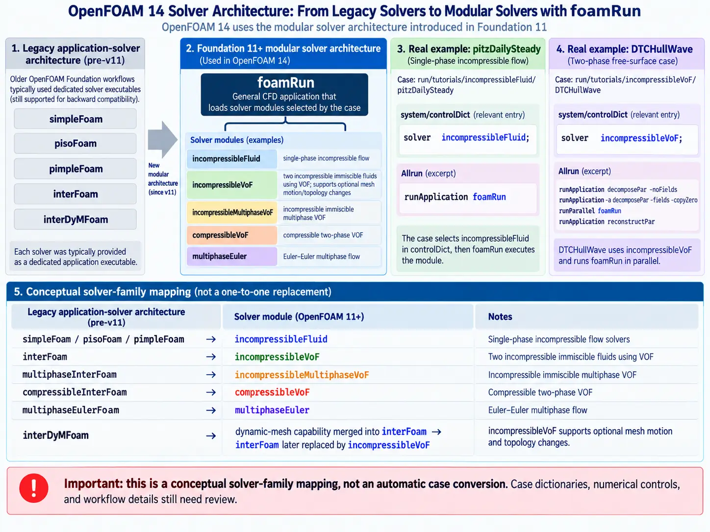
After understanding traditional solvers, modular architecture, foamRun, and solver capabilities, the next step is to examine how these components interact in a complete OpenFOAM 14 workflow.
The modular architecture does not replace the traditional OpenFOAM case structure. Instead, it introduces an additional organizational layer between case configuration and the numerical solution process.
A complete workflow can be represented as:
Each layer has a specific responsibility.
Understanding this separation helps users create, modify, and troubleshoot complex CFD simulations.
8.1 OpenFOAM Case Configuration
Every OpenFOAM simulation begins with a case directory.
The fundamental structure remains:
case/
0/constant/system/The modular architecture does not replace these directories.
Instead, the solver workflow uses the information provided by them.
The three directories define different aspects of the simulation:
| Directory | Purpose |
|---|---|
| 0/ | Initial and boundary conditions |
| constant/ | Mesh and physical definitions |
| system/ | Numerical and runtime controls |
Together, these files describe the engineering problem that will be solved.
8.2 Initial and Physical Definition Layer
The 0/ directory defines the initial state of the simulation.
Depending on the problem type, it may contain fields such as:
- velocity,
- pressure,
- phase fraction fields.
For example:
A single-phase flow case may require velocity and pressure fields.
A free-surface multiphase case may additionally require phase fraction information.
These fields define:
- initial conditions,
- inlet and outlet behaviour,
- wall conditions,
- interface states.
The constant/ directory defines the physical environment.
It contains information related to:
- computational mesh,
- material properties,
- physical models.
The mesh defines the computational domain through:
- cells,
- faces,
- boundaries,
- regions.
Physical properties define the behaviour of the simulated materials, including:
- density,
- viscosity,
- phase properties.
The accuracy of the CFD solution still depends strongly on appropriate mesh quality and physical modelling.
8.3 Numerical Control Layer
The system/ directory defines how the governing equations are solved.
Important files include:
controlDict,fvSchemes,fvSolution.
These files control:
- simulation time advancement,
- numerical discretization,
- linear solver settings,
- convergence criteria.
The numerical configuration remains essential regardless of whether the workflow uses traditional solver applications or modular capabilities.
8.4 Execution Framework Layer
Above the case configuration is the execution layer.
In the modular workflow, this role is provided by:
foamRun
The execution framework connects the prepared case with the selected solver capability.
The relationship is:
foamRunThe important architectural change is the separation between execution and physics.
The execution framework manages how the simulation runs.
The solver capability defines what type of CFD problem is being solved.
8.5 Solver Capability Layer
The solver module provides the computational framework required for a specific class of CFD problems.
Examples include:
| Capability | Application Area |
|---|---|
incompressibleFluid | Single-phase incompressible flow |
incompressibleVoF | Free-surface and VOF simulations |
multiphaseEuler | Eulerian multiphase systems |
A solver capability alone does not define the complete simulation.
The final behaviour depends on:
- physical models,
- material properties,
- boundary conditions,
- numerical settings.
8.6 Physical Model Layer
The physical model layer describes the behaviour of the simulated system.
Examples include:
Turbulence Models
Represent turbulent effects through approaches such as:
- RANS,
- LES.
Phase Models
Represent multiphase behaviour, including:
- interface capturing,
- phase interaction.
Transport Models
Define material behaviour through properties such as:
- viscosity,
- density,
- diffusion characteristics.
The separation of these models from the execution framework is one of the key advantages of modular organization.
8.7 Numerical Solution Layer
The final stage is the conversion of governing equations into a computational solution.
OpenFOAM performs this process through:
- spatial discretization,
- temporal discretization,
- algebraic equation solving,
- convergence monitoring.
The quality of the final CFD result depends on the interaction between:
No single component independently determines simulation accuracy.
8.8 Complete Workflow Example: DTC HullWave
The DTC HullWave case demonstrates how multiple layers interact within the modular workflow.
The architecture can be represented as:
foamRunincompressibleVoFThis example demonstrates that the geometry alone does not define the simulation.
The final result depends on the interaction between:
- correct case configuration,
- appropriate solver capability,
- suitable physical models,
- reliable numerical settings.
8.9 Why This Architecture Matters
The complete OpenFOAM 14 architecture allows users to understand CFD simulations as a connected workflow rather than a collection of separate solver commands.
The workflow changes from:
to:
This approach is especially valuable for advanced engineering applications where multiple physical processes must interact within a single simulation.
The modular architecture provides a clearer framework for organizing complex CFD workflows while preserving the fundamental CFD principles that OpenFOAM users rely on.
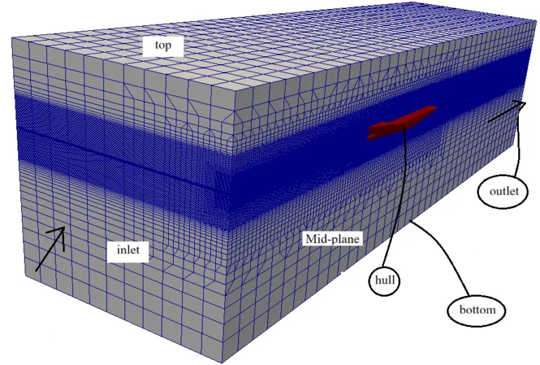
9. DTC HullWave Case Study: Applying OpenFOAM 14 Solver Architecture to Marine CFD
The transition from traditional solver applications toward modular solver architecture becomes clearer when applied to a realistic engineering problem.
The DTC HullWave case provides an example of how the OpenFOAM 14 workflow organizes a complex marine CFD simulation through the interaction of case configuration, solver capability, physical models, and numerical methods.
Marine hydrodynamics is a suitable example because ship-wave interaction involves several coupled physical processes:
Unlike a simple single-phase CFD problem, the simulation requires multiple capabilities to operate together within a single workflow.
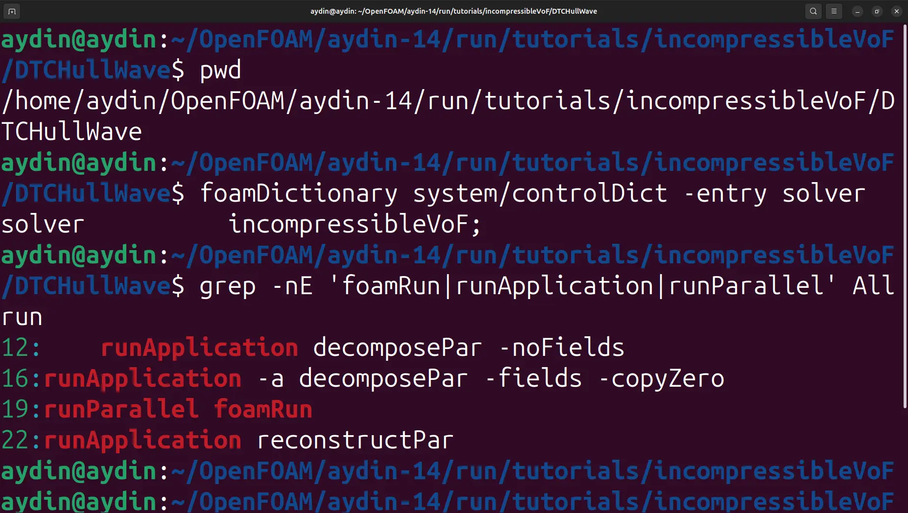
The DTC HullWave case represents a typical marine CFD problem where multiple physical capabilities must operate together, including incompressible flow modelling, free-surface tracking and turbulence simulation.
incompressibleVoF and free-surface modelling.9.1 Why DTC HullWave Represents a Complex CFD Problem
The DTC (Duisburg Test Case) hull is widely used as a benchmark geometry for ship hydrodynamics simulations.
The objective of such cases is to evaluate the ability of CFD methods to predict flow behaviour around a ship hull, including resistance, pressure distribution, and free-surface effects.
The complexity of the problem comes from the interaction of several physical phenomena.
Incompressible Flow Around the Hull
At typical ship operating conditions, water can generally be treated as an incompressible fluid.
The simulation must resolve:
- velocity distribution,
- pressure variation,
- flow separation,
- viscous effects.
Free-Surface Interaction
The water-air interface is one of the defining features of ship hydrodynamics.
The interface changes because of:
- hull motion,
- wave generation,
- pressure variations,
- turbulent flow structures.
For this reason, a multiphase approach such as VOF is required.
Complete DTC HullWave workflow using the OpenFOAM 14 modular solver architecture.
9.2 Traditional Solver-Based Interpretation
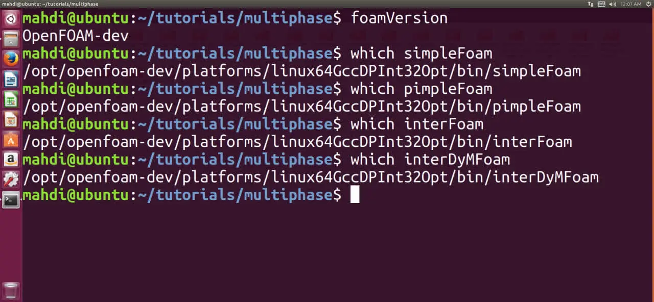
In the traditional OpenFOAM workflow, a user would typically begin by selecting a solver application associated with the required physics.
The workflow would be:
interFoamThe solver application represented the complete computational framework.
The user then configured:
- mesh,
- boundary conditions,
- physical properties,
- turbulence models,
- numerical schemes.
This workflow was effective and remains an important part of OpenFOAM history.
However, the solver name alone does not describe all the capabilities required by the simulation.
9.3 DTC HullWave in the Modular Workflow
The modular workflow begins by identifying the computational requirements of the problem.
For the DTC HullWave case, the required capabilities include:
- incompressible flow,
- two-phase interface tracking,
- VOF modelling,
- turbulence modelling,
- transient solution procedures.
The workflow becomes:
incompressibleVoFfoamRun ExecutionThe physical problem has not changed.
The governing equations, turbulence modelling, and interface treatment remain the same.
The difference is the way these capabilities are organized inside the software architecture.
9.4 Mapping Case Configuration to Marine CFD Requirements
The modular architecture still relies on the standard OpenFOAM case structure.
For the DTC HullWave simulation:
| Case Layer | Marine CFD Role |
|---|---|
| 0/ | Velocity, pressure, phase fraction fields |
| constant/ | Hull mesh, fluid properties, physical models |
| system/ | Time control, discretization, solver settings |
The case configuration provides the information required by the solver workflow.
The modular architecture determines how these components are connected during execution.
9.5 Complete DTC HullWave Workflow
The complete workflow can be represented as:
foamRunincompressibleVoFThis demonstrates the interaction between:
- case definition,
- execution framework,
- solver capability,
- physical models,
- numerical solution.
9.6 Practical Workflow for Engineers
A typical engineering workflow for a DTC HullWave simulation can be summarized as:
Step 1: Define the Physical Problem
Identify:
- hull geometry,
- operating conditions,
- fluid phases,
- expected flow behaviour.
Step 2: Select Required Capabilities
Determine:
- incompressible flow requirements,
- VOF interface modelling,
- turbulence approach,
- transient solution requirements.
Step 3: Configure the Case
Prepare:
- computational mesh,
- boundary conditions,
- physical properties,
- numerical schemes.
Step 4: Execute and Validate
Evaluate:
- wave pattern,
- resistance prediction,
- pressure distribution,
- convergence behaviour.
9.7 Why This Case Demonstrates the Value of Modular Architecture
The DTC HullWave case illustrates why separating execution from physical capability is useful.
A ship-wave interaction simulation is not defined by one physical model alone.
It requires the combination of:
- fluid flow,
- multiphase modelling,
- interface tracking,
- turbulence,
- transient calculation,
- numerical stability.
The modular workflow provides a way to organize these requirements without creating a separate solver application for every possible combination.
The focus changes from:
Which solver application represents this problem?
to:
Which computational capabilities are required to solve this problem?
9.8 Summary
The DTC HullWave case demonstrates how OpenFOAM 14 modular solver architecture can be applied to a realistic marine CFD problem.
The traditional workflow focused on selecting a complete solver application.
The modular workflow focuses on identifying required capabilities and connecting them through the execution framework.
For marine free-surface simulations, this means combining:
- incompressible flow capability,
- VOF interface modelling,
- turbulence models,
- numerical controls,
- appropriate case configuration.
The physics of marine CFD remains unchanged.
The main evolution is the organization of the computational workflow used to solve increasingly complex engineering problems.
10. Migration Guide for Existing OpenFOAM Users: Moving Toward the Modular Workflow
The transition from traditional OpenFOAM solver applications to the modular
workflow does not require users to replace their existing CFD knowledge.
The fundamental principles of OpenFOAM remain unchanged.
Users still need to understand:
- governing equations,
- mesh generation,
- boundary conditions,
- physical modelling,
- turbulence selection,
- numerical stability,
- convergence analysis.
The main change is the organization of solver functionality.
Previously:
Modular workflow:
Migration should therefore be understood as an architectural transition in software organization rather than a change in CFD methodology.
10.1 What Actually Changes During Migration
An important point for existing users is that not every part of an OpenFOAM case changes.
The traditional case structure remains:
case/
0/constant/system/These directories continue to define:
- field data,
- physical properties,
- mesh information,
- numerical controls.
The main change occurs in the relationship between:
- solver execution,
- solver capability,
- physical models.
Migration is therefore not a complete reconstruction of the CFD model.
The goal is to ensure that the selected capability matches the physical requirements of the case.
10.2 Step 1: Identify the Physical Requirements
The first step is moving away from solver-name-based thinking.
Traditional approach:
I need interFoam because this is a free-surface problem.
Capability-based approach:
This problem requires incompressible flow, interface tracking, and multiphase modelling.
For example, a ship hydrodynamics case requires:
These requirements determine the required solver capability.
10.3 Step 2: Relate Existing Solver Knowledge to Capabilities
Previous OpenFOAM experience remains valuable.
Traditional solvers already represent important CFD concepts.
Examples:
| Traditional Solver | Related Capability |
|---|---|
simpleFoam | incompressible single-phase flow |
interFoam | incompressible VOF capability |
pimpleFoam | transient incompressible workflow |
However, these relationships should not be interpreted as automatic conversions.
A solver application represents more than a name.
A complete CFD case also contains:
- field definitions,
- physical properties,
- boundary conditions,
- numerical schemes,
- model selections.
Migration requires checking the consistency of all these components.
10.4 Step 3: Review Case Configuration
After identifying the required capability, the existing case should be reviewed.
A practical migration checklist is:
| Case Component | Verification |
|---|---|
| 0/ | Required fields and boundary conditions |
| constant/ | Physical properties and models |
| system/ | Numerical settings and controls |
Field Definitions
The 0/ directory should be checked for:
- required fields,
- initial conditions,
- boundary conditions.
For multiphase cases, phase fields require special attention.
For example, in a water-air simulation:
alpha.water
must represent the intended initial interface distribution.
Physical Models
The constant/ directory should be reviewed for:
- fluid properties,
- turbulence models,
- phase models,
- transport properties.
Selecting a solver capability does not automatically create the required physical configuration.
Numerical Settings
The system/ directory remains essential.
Important files include:
controlDict,fvSchemes,fvSolution.
These define:
- time control,
- discretization,
- linear solver settings,
- convergence criteria.
10.5 Step 4: Validate the Migrated Case
A successful migration means more than completing a simulation run.
The results must still represent the expected physical behaviour.
Validation should include:
Numerical Checks
- residual behaviour,
- time-step stability,
- convergence trends.
Physical Checks
- expected flow pattern,
- pressure distribution,
- interface behaviour,
- conservation properties.
Comparison
When available, compare results with:
- previous simulations,
- benchmark cases,
- experimental measurements.
10.6 Common Migration Mistakes
Mistake 1: Treating Modules as Direct Solver Replacements
A common misunderstanding is:
The relationship is based on capability, not direct replacement.
Mistake 2: Ignoring Physical Configuration
Selecting a capability does not automatically define:
- turbulence,
- material properties,
- phase behaviour,
- numerical schemes.
These still require correct configuration.
Mistake 3: Focusing Only on Software Changes
The modular architecture changes software organization.
It does not replace the importance of:
- mesh quality,
- physical modelling,
- numerical stability,
- validation.
10.7 Recommended Learning Path
For users familiar with traditional OpenFOAM workflows, the transition can be approached incrementally.
The recommended path is:
foamRun WorkflowUsers who already understand:
- case structure,
- solver settings,
- physical modelling,
- numerical methods,
- already possess the foundation required for the modular workflow.
10.8 Summary
Migration toward the OpenFOAM 14 modular workflow should be understood as an architectural transition.
The user moves from selecting a complete solver application toward identifying the computational capability required by the physical problem.
The main migration steps are:
- Define the physical requirements.
- Identify the appropriate solver capability.
- Review case configuration.
- Validate the simulation results.
The modular workflow preserves existing CFD knowledge while providing a more flexible way to organize increasingly complex OpenFOAM simulations.
11. Frequently Asked Questions About OpenFOAM 14 Solver Architecture
This section addresses the most common questions related to the transition from traditional OpenFOAM solver applications toward the modular solver architecture introduced in OpenFOAM 14.
The purpose is to clarify the relationship between existing OpenFOAM knowledge, foamRun, solver modules, and the new capability-based workflow.
Does OpenFOAM 14 require existing users to relearn CFD?
No.
The transition to modular solver architecture does not change the CFD
principles used in OpenFOAM.
Existing knowledge of:
- governing equations,
- mesh generation,
- physical modelling,
- numerical methods,
- convergence analysis
- remains essential.
The main change is how solver functionality is organized within the software framework.
Is foamRun a replacement for traditional solvers?
No.
foamRun should not be considered a new universal CFD solver or a direct replacement for applications such as:
simpleFoam,pimpleFoam,interFoam.
Its role is to provide the execution framework required to run solver modules.
The relationship is:
foamRunThe solver module defines the CFD capability, while foamRun manages the execution process.
Are traditional solvers such as simpleFoam and interFoam still relevant?
Yes.
Traditional solver applications remain important because they represent the historical organization of OpenFOAM workflows and provide the foundation for understanding the corresponding CFD capabilities.
Examples include:
simpleFoam— steady incompressible flow workflows,pimpleFoam— transient incompressible flow workflows,interFoam— incompressible VOF free-surface workflows.
The modular architecture does not remove this knowledge.
Instead, it reorganizes these concepts into a capability-based framework.
Do solver modules directly replace old solvers?
No.
Solver modules should not be interpreted as one-to-one replacements for traditional solver applications.
The relationship is based on computational functionality rather than direct conversion.
| Traditional Solver | Related Capability |
|---|---|
simpleFoam | Incompressible flow capability |
pimpleFoam | Incompressible flow capability with transient solution configuration |
interFoam | Incompressible VOF capability |
multiphaseEulerFoam | Eulerian multiphase capability |
These relationships provide a conceptual mapping between workflows, but they do not represent automatic case conversion.
Do existing OpenFOAM cases need to be rebuilt?
Not necessarily.
The fundamental OpenFOAM case structure remains:
case/
0/constant/system/Existing cases still contain essential information:
- field definitions,
- boundary conditions,
- physical properties,
- numerical settings.
However, migration requires verifying that the case configuration is compatible with the selected solver capability.
Important areas include:
- required fields,
- physical models,
- phase definitions,
- turbulence settings,
- numerical schemes.
The objective is not to recreate the entire CFD model, but to ensure consistency between the existing case and the modular workflow.
Does modular architecture automatically improve CFD accuracy?
No.
Modular architecture changes the organization of CFD software components. It does not automatically improve numerical accuracy.
The quality of a CFD simulation still depends on:
- mesh quality,
- appropriate physical models,
- boundary conditions,
- numerical schemes,
- convergence behaviour,
- validation methodology.
A more flexible software architecture does not replace correct CFD practice.
Why is modular architecture useful for complex simulations?
Modern engineering simulations often require several interacting capabilities.
Examples include:
- ship hydrodynamics,
- multiphase industrial flows,
- moving-body simulations,
- transient multiphysics applications.
In an application-based workflow, supporting every possible combination of requirements can result in an increasing number of specialized solver applications.
The modular approach separates:
This provides a more flexible structure for organizing complex CFD workflows.
Can old OpenFOAM tutorials still be useful?
Yes.
Traditional tutorials remain valuable because they explain fundamental CFD concepts, including:
- case preparation,
- physical modelling,
- boundary conditions,
- numerical settings,
- validation procedures.
However, when adapting older tutorials, users should focus on the physical requirements of the problem rather than only the historical solver name.
For example, an interFoam tutorial remains valuable because it explains:
- VOF modelling,
- phase fraction fields,
- multiphase boundary conditions.
These concepts remain relevant within a modular workflow.
What should existing users focus on when migrating?
A practical migration strategy consists of four steps:
1. Understand the physical problem
Identify:
- flow regime,
- phases involved,
- turbulence requirements,
- transient behaviour.
2. Identify the required capability
Select the solver capability that represents the required computational framework.
3. Review the case configuration
Check:
- fields,
- physical models,
- numerical settings.
4. Validate the results
Evaluate:
- convergence behaviour,
- physical trends,
- previous simulations,
- benchmark results when available.
Final Summary
The transition to OpenFOAM 14 modular solver architecture represents a change in how solver functionality is organized.
The key concepts are:
foamRunprovides the execution framework.- Solver modules provide CFD capabilities.
- Physical models define system behaviour.
- Numerical settings control solution procedures.
Traditional OpenFOAM knowledge remains fully relevant.
The main conceptual transition is moving from:
toward:
The modular workflow provides a more flexible organization of OpenFOAM simulations while preserving the engineering principles that form the foundation of CFD.
12. Conclusion: Understanding OpenFOAM 14 Solver Architecture
OpenFOAM 14 represents an important evolution in the organization of CFD workflows. This evolution is not a change in the fundamental principles of computational fluid dynamics, governing equations, or numerical solution methods. Instead, it introduces a different way of structuring how computational capabilities are assembled, executed, and extended within the OpenFOAM framework.
For many years, OpenFOAM users interacted with the software through dedicated solver applications such as simpleFoam, pimpleFoam, and interFoam. These applications provided complete computational workflows by combining numerical procedures, physical models, and solution strategies into individual solver executables. This approach was effective and established a clear relationship between a class of physical problems and a corresponding solver application.
However, the increasing complexity of modern engineering simulations has created new requirements. Advanced CFD applications often involve multiple interacting capabilities, including multiphase modelling, turbulence treatment, transient flow behaviour, moving boundaries, and specialized numerical approaches. The main challenge is no longer only solving individual physical problems, but organizing these different capabilities in a flexible and maintainable framework.
The modular solver architecture addresses this challenge by separating the main components of the simulation workflow:
foamRunWithin this structure, foamRun provides the execution framework, while solver modules define the computational capabilities required for different categories of CFD problems. Physical models and numerical settings remain essential components that determine the final behaviour and accuracy of the simulation.
The central conceptual transition is therefore a move from an application-based mindset toward a capability-based approach.
The traditional question:
Which solver application should I run?
is replaced by a more fundamental question:
Which computational capabilities does my physical problem require?
The DTC HullWave marine CFD case demonstrates this transition clearly. A ship free-surface simulation is not defined only by a solver name. It requires the combination of incompressible flow modelling, VOF interface capturing, turbulence modelling, transient solution procedures, wave conditions, and appropriate numerical controls. The modular workflow provides a structured method for connecting these requirements within a single simulation framework.
For existing OpenFOAM users, this transition builds upon previous CFD experience rather than replacing it. Knowledge of mesh generation, boundary conditions, physical modelling, numerical schemes, and convergence analysis remains essential. The main conceptual shift is understanding how these components are organized within the modular architecture.
The modular solver approach extends the original OpenFOAM philosophy of flexibility, transparency, and user control by providing a more scalable framework for increasingly complex CFD applications. By separating execution, solver capabilities, physical models, and numerical methods, OpenFOAM 14 provides a clearer architecture for developing, adapting, and understanding advanced simulation workflows.
Ultimately, understanding this architectural transition allows users to move beyond selecting predefined solver applications and toward a deeper understanding of how CFD capabilities are combined to represent complex engineering problems.
For users preparing their CFD environment, see our OpenFOAM on Ubuntu 24.04 Installation Guide.