
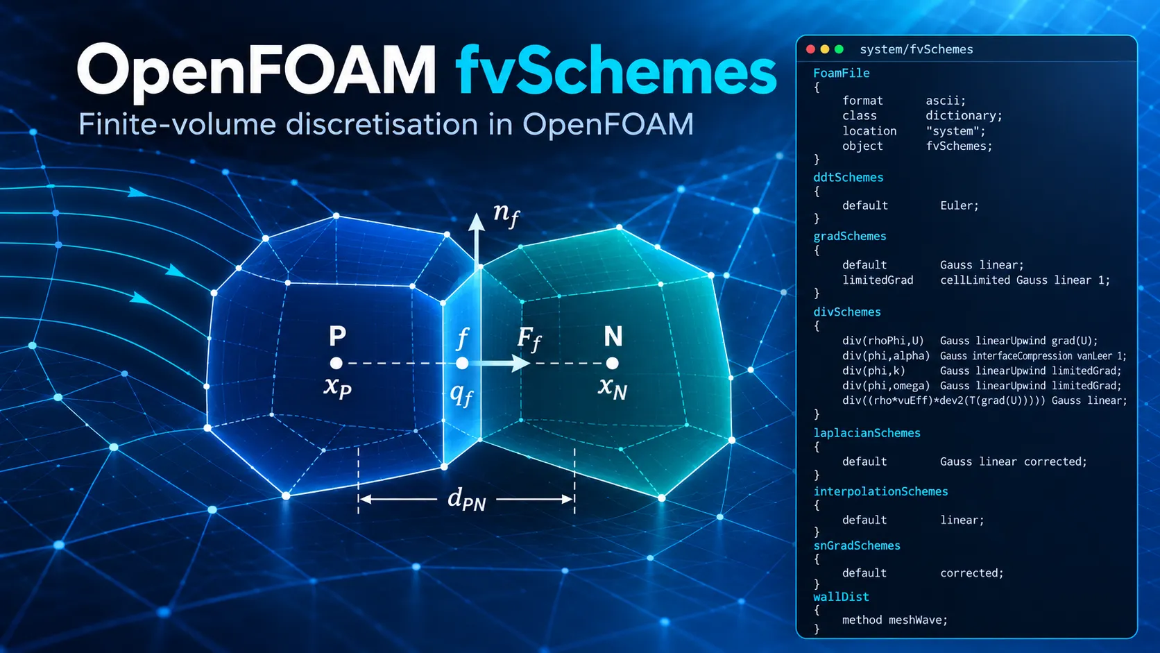
OpenFOAM fvSchemes in Foundation 14
In OpenFOAM, system/fvSchemes specifies the numerical schemes used to discretise time derivatives, gradients, divergence terms, Laplacians, cell-to-face interpolation and surface-normal gradients. [1] [2]
This guide uses OpenFOAM Foundation 14 terminology and the supplied Foundation 14 dictionary as its working example. It explains what each entry means, how related entries interact, and how the documented scheme properties connect to marine CFD practice and numerical verification. [1] [16] [17]
The article does not present a universal fvSchemes file. Release-specific syntax and scheme availability should be checked against the exact OpenFOAM distribution and solver being used. [1]
For related background, see Ocean Tech Review’s OpenFOAM 14 case structure guide, OpenFOAM 14 controlDict guide, and OpenFOAM 14 solver architecture. If you are new to running Foundation 14 cases, start with the pitzDailySteady tutorial.
1. What fvSchemes Controls
The fvSchemes file resides in the system directory. In a standard OpenFOAM case, system also contains controlDict, which controls run and output settings, and fvSolution, which contains equation-solver and algorithm controls. [1] [18]
| Dictionary | Operation | What It Controls |
|---|---|---|
ddtSchemes | First time derivatives | Temporal discretisation. |
gradSchemes | Gradients | Cell-gradient reconstruction. |
divSchemes | Divergence terms | Convection and other general divergence operators. |
laplacianSchemes | Laplacians | Diffusion-type operators and their surface-normal-gradient treatment. |
interpolationSchemes | Cell-to-face interpolation | General evaluation of face values. |
snGradSchemes | Surface-normal gradients | Normal derivatives at faces. |
The Foundation 14 dictionary used as the working example in this article is:
FoamFile
{
    format      ascii;
    class       dictionary;
    location    "system";
    object      fvSchemes;
}

ddtSchemes
{
    default         Euler;
}

gradSchemes
{
    default         Gauss linear;
    limitedGrad     cellLimited Gauss linear 1;
}

divSchemes
{
    div(rhoPhi,U)   Gauss linearUpwind grad(U);
    div(phi,alpha)  Gauss interfaceCompression vanLeer 1;
    div(phi,k)      Gauss linearUpwind limitedGrad;
    div(phi,omega)  Gauss linearUpwind limitedGrad;
    div(((rho*nuEff)*dev2(T(grad(U))))) Gauss linear;
}

laplacianSchemes
{
    default         Gauss linear corrected;
}

interpolationSchemes
{
    default         linear;
}

snGradSchemes
{
    default         corrected;
}

wallDist
{
    method meshWave;
}
This is a specific Foundation 14 configuration, not a universal fvSchemes template. OpenFOAM’s own guidance is to start from tutorials relevant to the solver and physical problem being used. [1]
2. The Finite-Volume Meaning of a Numerical Scheme
Consider a transported quantity q:
∂(ρq)/∂t + ∇·(ρu q) = ∇·(Γ∇q) + Sq.
Here, ρ is density, u is velocity, Γ is a diffusion coefficient and Sq represents source terms.
Finite-volume discretisation integrates the governing equation over each control volume. A representative convective contribution for a cell P can be written as (1/VP) Σf Ff qf, where Ff = (ρu)f · Sf. The divergence theorem converts volume integrals of divergence terms into sums of fluxes over cell faces. [2]
Because field values are principally stored at cell centres while flux calculations require face values, a numerical scheme is required to construct or interpolate qf. This is the role of schemes such as upwind, linear, linearUpwind and limited interpolation schemes. [1] [2] [5] [6] [7]
3. Reading phi and rhoPhi Correctly
In OpenFOAM, phi is a face-flux field whose precise dimensions and physical meaning depend on the governing formulation. The supplied dictionary contains:
div(rhoPhi,U)   Gauss linearUpwind grad(U);
div(phi,alpha)  Gauss interfaceCompression vanLeer 1;
The Foundation 14 damBreakLaminar documentation uses these same operator names: div(rhoPhi,U) for momentum convection and div(phi,alpha) for phase transport. [12]
Consequently, div(phi,U) and div(rhoPhi,U) should not be substituted for one another merely because both describe a convective divergence involving velocity. The lookup must match the equation assembled by the selected solver or solver module.
For the wider solver-module context, see Ocean Tech Review’s OpenFOAM 14 Solver Architecture.
4. ddtSchemes: Time Discretisation
The example uses:
ddtSchemes
{
    default    Euler;
}
Euler
For a constant time step, the implicit Euler approximation is (qn+1 − qn)/Δt. Foundation 14 documents Euler as a transient, first-order implicit scheme, and the documented Foundation 14 damBreakLaminar tutorial uses it. [1] [12]
The time scheme does not determine the time-step size. deltaT, automatic time-step adjustment and Courant-number limits belong to controlDict. [12] [18] See the Ocean Tech Review OpenFOAM 14 controlDict guide.
Backward
Foundation 14 documents backward as an implicit second-order time scheme. For constant Δt, the derivative is represented by (3qn+1 − 4qn + qn−1)/(2Δt). The constant-step expression is not the mathematical description of the variable-time-step form. [1] [11]
Crank–Nicolson
ddtSchemes
{
    default    CrankNicolson 0.9;
}
In Foundation 14, the off-centering coefficient ranges from 0, corresponding to Euler, to 1, corresponding to pure Crank–Nicolson. The User Guide states that 0.9 is generally used to stabilise the scheme in practical engineering applications. [1]
The formal order of a time scheme does not establish the temporal accuracy of the entire simulation. The selected Δt, physical time scales and other discretisation errors remain part of the numerical problem. [11] [17]
5. gradSchemes: Gradient Reconstruction
The example defines:
gradSchemes
{
    default         Gauss linear;
    limitedGrad     cellLimited Gauss linear 1;
}
Gauss linear
For a scalar q, the Gauss gradient can be represented as (∇q)P ≈ (1/VP) Σf qfSf. Foundation 14 describes Gauss linear as the standard Gauss gradient with linear interpolation from cell centres to face centres. [1] [3]
cellLimited Gauss linear 1
cellLimited limits extrapolated face values so that they do not exceed the range defined by the cell and surrounding-cell values. For the limiter coefficient, 1 requests full limiting and 0 removes limiting. [1] [4] [13]
The source documentation describes cellLimitedGrad as a limiter applied to a run-time-selected base gradient scheme, with the scalar limiter applied to all gradient components. [13]
6. linearUpwind and Its Dependence on the Gradient
The momentum entry is:
div(rhoPhi,U) Gauss linearUpwind grad(U);linearUpwind starts from the upwind cell and adds an explicit gradient-based correction. Conceptually, qf ≈ qup + (∇q)up · (xf − xup). OpenFOAM Foundation documentation classifies linearUpwind as second-order, upwind-biased and unbounded. [1] [6]
The turbulence transport entries instead use the named gradient:
div(phi,k)      Gauss linearUpwind limitedGrad;
div(phi,omega)  Gauss linearUpwind limitedGrad;
The distinction is important: changing the gradient treatment can change a linearUpwind reconstruction even when the word linearUpwind itself is unchanged. [4] [6]
7. divSchemes: Divergence and Convection
The divSchemes dictionary contains divergence terms. Many important entries are convection operators, although general divergence terms can also appear here. [1] [2]
| Scheme | Documented Character | Main Numerical Point |
|---|---|---|
upwind | First-order, bounded | Robust but numerically diffusive. [1] [5] |
linear | Second-order, unbounded | Lower dissipation but can generate unbounded advection solutions. [1] [2] |
linearUpwind | Second-order, upwind-biased, unbounded | Uses an explicit gradient correction. [1] [6] |
limitedLinear | Limited linear/upwind family | Moves toward upwind as limiting strengthens. [1] [7] |
First-order upwind
div(phi,U) Gauss upwind;Upwind uses the value in the cell upstream of the face. Its leading spatial truncation error contains a diffusion-like contribution, which explains its characteristic numerical diffusion. [1] [5]
For a one-dimensional uniform grid with positive constant velocity, (qi − qi−1)/Δx = ∂q/∂x − (Δx/2)∂²q/∂x² + O(Δx²). This isolates the spatial approximation; the complete error also depends on time discretisation, mesh geometry and the other equation terms. [2] [5]
ITTC’s 2024 ship-CFD guideline characterises first-order upwind as stable but strongly affected by artificial numerical diffusion and recommends second-order upwind treatment for convection-diffusion transport equations in its body-fitted ship-CFD guidance. [16]
Linear
div(phi,U) Gauss linear;Foundation 14 classifies linear convection as second-order and unbounded. Its lower numerical dissipation does not remove the need to examine stability, boundedness and resolution. [1] [2]
Limited linear and limitedLinearV
div(phi,U)    Gauss limitedLinear 1;
div(phi,U)    Gauss limitedLinearV 1;
limitedLinear retains linear interpolation where allowed by its limiter and moves toward upwind as limiting becomes stronger. Foundation 14 states that the coefficient 1 gives the strongest limiting and the scheme tends toward linear as the coefficient approaches zero. [1] [7]
For vector-specific V variants, Foundation 14 states that one limiter is calculated for the vector and applied to all components, based on the direction with the most rapidly changing gradient. [1]
8. The bounded Prefix
div(phi,U) bounded Gauss linearUpwind grad(U);The meaning of bounded here is specific. It concerns the relationship between conservative and advective forms. For constant-density incompressible flow, ∇·(u q) = u·∇q + q∇·u. The two forms become equivalent when the discrete continuity condition is satisfied. During an iterative steady-state calculation, continuity error may initially be significant, and OpenFOAM’s bounded advection treatment accounts for the associated contribution. As the continuity defect disappears, that correction disappears. [8]
9. Phase-Fraction Transport Is a Separate Numerical Problem
div(phi,alpha) Gauss interfaceCompression vanLeer 1;This entry should not be interpreted using the same rules as ordinary momentum convection. Foundation 14’s documented damBreakLaminar case uses the same form. Its incompressibleVoF solver uses MULES for phase-fraction transport, and the User Guide states that MULES maintains boundedness of the phase fraction. interfaceCompression provides dedicated interface compression while vanLeer supplies the associated limited interpolation. [12]
Foundation 14 documents the interface-compression coefficient as 0 for no compression, 1 for conservative compression, and values greater than 1 for enhanced compression. The documented damBreakLaminar case uses 1. [12]
For a VOF calculation, 0 ≤ α ≤ 1 is a boundedness requirement for the phase fraction. It is not by itself a measure of errors in wave amplitude, wave phase, pressure or hydrodynamic loading. Verification of those quantities is separate. [12] [17]
10. Turbulence Transport in the Example
div(phi,k)      Gauss linearUpwind limitedGrad;
div(phi,omega)  Gauss linearUpwind limitedGrad;
Both k and ω are convected with linearUpwind, while the gradient required by the explicit reconstruction is the named limitedGrad definition rather than the default Gauss linear gradient.
This demonstrates why an fvSchemes file must be read as a connected set of definitions. A named gradient entry can be referenced by another discretisation scheme. [1] [4] [6]
The suitability of a particular turbulence-transport discretisation is case-dependent. Foundation documentation recommends using relevant tutorials as the starting reference rather than treating one dictionary as universally applicable. [1]
11. General Divergence Terms
div(((rho*nuEff)*dev2(T(grad(U))))) Gauss linear;This is not another ordinary advection entry. OpenFOAM also uses divSchemes for general divergence operators. CFD Direct’s finite-volume documentation distinguishes such general divergence terms from advection and Laplacian operators and describes their Gauss discretisation through a surface sum with face interpolation. [2]
Therefore, the meaning of Gauss linear must always be interpreted in the context of the complete operator to which it is applied.
12. laplacianSchemes
laplacianSchemes
{
    default    Gauss linear corrected;
}
For a diffusion-type operator ∇·(Γ∇q), finite-volume discretisation requires both the coefficient at the face and the surface-normal gradient. [9]
Foundation 14 therefore specifies Laplacian schemes using the form Gauss <interpolationScheme> <snGradScheme>. Documented examples include Gauss linear corrected, Gauss linear limited corrected 0.33, Gauss linear limited corrected 0.5, Gauss linear orthogonal and Gauss linear uncorrected. [1]
In Gauss linear corrected, linear interpolates the diffusion coefficient to the face, while corrected specifies the surface-normal-gradient treatment. The word corrected refers to geometric non-orthogonality correction; it does not mean the complete discretisation has been corrected for every source of numerical error. [1] [9] [10]
13. snGradSchemes and Non-Orthogonality
snGradSchemes
{
    default    corrected;
}
The surface-normal gradient approximates the derivative normal to a face. For an orthogonal face, the line joining neighbouring cell centres is aligned with the face-normal direction. On a non-orthogonal face, the directions differ, and the corrected formulation adds an explicit contribution associated with that non-orthogonality. [10]
Foundation 14 also provides limited correction:
snGradSchemes
{
    default    limited corrected 0.5;
}
The Foundation 14 source documentation defines 0 as switching the correction off, 1 as permitting the full selected correction, and 0.5 as limiting the non-orthogonal contribution so that it does not exceed the orthogonal contribution. Thus, 0.5 does not mean that half of the correction is uniformly applied at every face. [14]
The same syntax can appear directly inside a Laplacian specification. Because a Laplacian entry explicitly contains its surface-normal-gradient scheme, the complete Laplacian entry must be read when determining which correction is actually used. [1]
14. interpolationSchemes
interpolationSchemes
{
    default    linear;
}
For adjacent cells P and N, linear cell-to-face interpolation can be represented as qf = wfqP + (1−wf)qN. The weight is determined by mesh geometry and is not generally one half. [9]
Foundation 14 reports that linear is the default interpolation scheme used in almost all tutorial cases. One principal use is evaluating velocity at face centres for construction of the flux field. [1]
The general interpolation default does not replace a scheme explicitly specified inside another operator. For example, div(rhoPhi,U) Gauss linearUpwind grad(U); continues to use linearUpwind even when the general interpolation default is linear. [1]
15. wallDist Is Not a Discretisation Scheme
wallDist
{
    method meshWave;
}
This block is stored in fvSchemes, but it does not select the discretisation of a differential operator. Foundation 14 source documentation defines wallDist as the interface to run-time-selectable methods for calculating distance-to-wall and, optionally, normal-to-wall fields. meshWave, Poisson and advectionDiffusion are among the available distance methods. [15]
method meshWave; should therefore be read as a wall-distance calculation choice, not as another interpolation or derivative scheme. [15]
16. Accuracy, Stability and Boundedness Are Different Properties
Accuracy
For a sufficiently smooth problem in an asymptotic refinement range, a spatial error contribution can be represented as Eh ≈ Chhp, and a temporal contribution as Et ≈ Ct(Δt)r. The formal order of one scheme does not establish the observed convergence order of a complete CFD simulation. [2] [17]
Stability
Stability concerns the growth or control of numerical disturbances. A stable calculation is not necessarily accurate. First-order upwind, for example, is documented as bounded and robust but also introduces substantial artificial diffusion. [1] [5]
Boundedness
Different uses of the word bounded must be kept separate: first-order upwind has a boundedness property subject to its transport assumptions; cellLimited bounds extrapolated gradient reconstruction; the bounded divergence prefix addresses conservative versus advective discretisation in the presence of continuity error; and MULES provides specialised bounded phase-fraction transport. [5] [1] [4] [8] [12]
17. What “Second Order” Does and Does Not Mean
A method described as second order has a truncation-error relationship under specified mathematical assumptions. It does not mean that the final engineering result is automatically twice as accurate as the result from a first-order method. [2] [17]
Foundation 14 classifies linearUpwind as second-order and upwind-biased, but also as unbounded. Likewise, backward and CrankNicolson are documented as second-order time schemes, but their formal order does not determine whether a selected Δt resolves a particular transient event. [1] [11]
Formal order is a property of a discretisation under its assumptions; observed convergence belongs to the complete numerical solution and must be measured. [17]
18. Time-Step Size Is Separate from the Time Scheme
A basic advective Courant number can be expressed as Co ≈ UΔt/Δx. Foundation 14 uses Courant-number control in its documented transient VOF tutorial and distinguishes the time-integration scheme from time-step control. [12]
For marine CFD, relevant physical time scales can include a wave period, rotational period, blade-passing period or impact-event duration. ITTC treats the time step as a separate numerical consideration from the spatial discretisation schemes. [16]
Consequently, selecting Euler or a higher-order alternative does not by itself establish adequate temporal resolution.
19. Marine CFD Interpretation
ITTC’s 2024 Practical Guidelines for Ship CFD Applications states that diffusion terms in most industrial CFD codes are normally treated with second-order central differencing, making convection discretisation a major determinant of spatial accuracy. The guideline describes first-order upwind as stable but numerically diffusive and identifies second-order upwind schemes as an industrial workhorse for body-fitted convection-diffusion calculations. [16]
The same guideline distinguishes turbulence-resolving calculations such as LES and DNS, where low numerical dissipation becomes particularly important, from conventional RANS applications. [16]
These are general ship-CFD guidelines, not a universal OpenFOAM dictionary. Within Foundation 14, the relevant tutorial and exact solver formulation remain the appropriate starting points for valid entries. [1]
20. Free-Surface Marine CFD
Foundation 14’s documented VOF configuration illustrates why a free-surface fvSchemes file cannot be reduced to one preferred convection scheme:
div(phi,alpha)    Gauss interfaceCompression vanLeer 1;
div(rhoPhi,U)     Gauss linearUpwind grad(U);
MULES maintains phase-fraction boundedness, while interface compression controls the numerical treatment of the fluid interface. Momentum transport is discretised separately. [12]
For marine applications, bounded phase fraction and accurate hydrodynamic prediction are distinct questions. A free-surface calculation can satisfy phase-fraction bounds while still containing discretisation error in resistance, pressure, wave elevation or phase. Those quantities require their own numerical verification. [17]
21. Verification of an fvSchemes Choice
ITTC distinguishes verification, validation and uncertainty assessment. Solution verification concerns estimation of numerical error in the computational solution, while validation concerns comparison with physical reality using experimental information and associated uncertainties. [17]
For discretisation studies, ITTC describes systematic use of multiple grid resolutions and discusses methods including Stern et al. and Eça–Hoekstra. The Stern procedure uses three grids for its leading-term estimate; the Eça–Hoekstra approach uses at least four grids and applies least-squares fitting to address scatter in practical CFD data. [17]
An fvSchemes comparison is therefore not verification merely because two settings give similar values. ITTC’s methodology requires the convergence behaviour of solution data to be examined rather than imposing an assumed convergence rate on data that do not support it. [17]
22. Reading the Example Dictionary as a Whole
| Entry | Interpretation |
|---|---|
default Euler; | Default first-time derivatives use first-order implicit Euler. [1] |
default Gauss linear; | Default gradient uses Gauss construction with linear face interpolation. [1] [3] |
limitedGrad cellLimited Gauss linear 1; | Defines a fully limited named gradient for operators that request limitedGrad. [1] [13] |
div(rhoPhi,U) ... linearUpwind grad(U) | Momentum convection uses second-order upwind-biased linearUpwind with a velocity-gradient correction. [1] [6] |
div(phi,alpha) ... interfaceCompression vanLeer 1 | Phase fraction uses the specialised VOF interface-compression formulation. [12] |
div(phi,k) / div(phi,omega) | Turbulence variables use linearUpwind with the named limited gradient. |
div(((rho*nuEff)*dev2(T(grad(U))))) Gauss linear; | General divergence term using Gauss discretisation and linear face interpolation. [2] |
Gauss linear corrected | Laplacians use Gauss discretisation, linear coefficient interpolation and corrected surface-normal gradients. [1] [9] [10] |
interpolationSchemes default linear; | General cell-to-face interpolation defaults to linear. [1] [9] |
snGradSchemes default corrected; | Default surface-normal gradients include explicit non-orthogonal correction. [10] |
wallDist method meshWave; | Wall distance is calculated with the meshWave method. [15] |
23. Common fvSchemes Questions
Is linearUpwind bounded?
No. Foundation 14 classifies linearUpwind as second-order, upwind-biased and unbounded. Gradient limiting can be applied to the reconstruction, but that is a separate numerical operation. [1] [4] [6]
Is upwind bounded?
Foundation 14 classifies standard upwind as first-order and bounded. CFD Direct notes that the boundedness argument for conservative advection depends on the relevant continuity condition. [1] [5]
Is linear always second order?
Foundation 14 classifies linear convection as second-order and unbounded. The observed order of a complete solution still depends on the full discretisation and refinement behaviour. [1] [17]
Does Gauss linear mean the same thing everywhere?
No. The role of linear depends on the operator: it can provide face interpolation for a gradient, interpolate a Laplacian coefficient, or supply face values for a general divergence term. [1] [2] [9]
Does corrected mean a more accurate solution in general?
No. In snGradSchemes and the surface-normal-gradient part of a Laplacian scheme, corrected specifically refers to correction for mesh non-orthogonality. [9] [10]
Does limited corrected 0.5 mean 50% correction?
No. Foundation 14 defines 0.5 so that the magnitude of the non-orthogonal correction does not exceed the orthogonal contribution. [14]
24. References
- OpenFOAM Foundation 14 User Guide — Numerical schemes
- Greenshields and Weller — Notes on Computational Fluid Dynamics: General Principles, Numerical Method
- Greenshields and Weller — Gradient discretisation
- Greenshields and Weller — Gradient limiting
- Greenshields and Weller — Upwind scheme
- Greenshields and Weller — Linear upwind scheme
- Greenshields and Weller — Useful TVD schemes
- Greenshields and Weller — Bounded advection discretisation
- Greenshields and Weller — Laplacian discretisation and interpolation
- Greenshields and Weller — Surface-normal gradient
- Greenshields and Weller — Second-order time schemes
- OpenFOAM Foundation 14 User Guide — Breaking of a dam
- OpenFOAM Foundation 14 Source Guide — cellLimitedGrad
- OpenFOAM Foundation 14 Source Guide — limitedSnGrad
- OpenFOAM Foundation 14 Source Guide — wallDist
- ITTC 2024 — Practical Guidelines for Ship CFD Applications, 7.5-03-02-03, Revision 02
- ITTC 2024 — Uncertainty Analysis in CFD, Verification and Validation Methodology and Procedures, 7.5-03-01-01, Revision 05
- OpenFOAM Foundation 14 User Guide — Case file structure
25. Choosing fvSchemes for the Engineering Result
The names inside fvSchemes identify numerical methods applied to specific operators. They do not, by themselves, establish that the resulting simulation is sufficiently accurate for a particular engineering quantity. [1] [17]
For marine CFD, ITTC guidance places particular attention on convection discretisation, time-step selection and systematic verification of the quantities of interest. Foundation 14 documentation, meanwhile, defines the syntax and properties of the schemes available in OpenFOAM. [16] [17] [1]
A defensible setup therefore begins with the exact solver formulation and a relevant Foundation 14 tutorial, then evaluates the numerical sensitivity of the engineering result that the calculation is intended to predict. [1] [17]